Oliver Heaviside and the theory of transmission lines

Pieter-Tjerk de Boer, PA3FWM web@pa3fwm.nl

(This is an adapted version of an article I wrote for the Dutch
amateur radio magazine Electron, November 2021.)

An antenna cable is not just a piece of wire.
Technically, it’s called a “transmission line”,
with special properties such as its characteristic impedance.
But transmission lines are quite a bit older than radio technology: they date back to the
second half of the 19th century, in the form of (mostly submarine) telegraph cables.
In this article we look at the principles and properties of transmission lines,
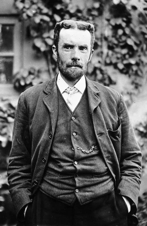
with special emphasis on Oliver Heaviside’s contribution to our knowledge of them.

Oliver Heaviside

After secondary school, Oliver Heaviside (1850-1925) started working at the company
which operated the submarine telegraph cable between Newcastle (UK) and Denmark.
At first he worked as a telegraph operator, but soon he also got involved with the
(electro)technical side of the telegraph systems.
One of the things he noticed, was that when water leaked into a submarine cable and
progressively short-circuited it, the signals did not just become weaker (as expected),
but also clearer, less distorted.

In those days, electrical engineering was still in its infancy.
Thanks to the work of physicists like Volta, Ampère, Ørsted and Faraday, there was a decent
understanding of generating electrical currents and moving compass needles using an electromagnet.
Together, that is enough for building a telegraph, at least in principle.
But if one uses as very long cable, and tries to send dots and dashes at a high rate,
it turned out to not work so well.
There was little theoretical understanding of this,
particularly among the more practically minded people who cobbled together telegraph systems.

Heaviside studied physics by himself, and stumbled on the books by James Clerk Maxwell.
Maxwell’s ideas about electromagnetism were, at that time, rather speculative and not widely accepted,
but Heaviside got enthousiastic, studied them, and succesfully applied this theory to telegraph lines.

Thus, Heaviside, who never had studied at a university, rose from being a humble telegraph operator
to a respected physicist.
After quitting his job at the telegraph company at the age of 24, he never had another job.
The rest of his life he lived in relative poverty while working on the theory.
He became one of the so-called Maxwellians: a group of physicists who enhanced Maxwell’s
theory after his untimely death (in 1879 at the age of 48) and popularised it.
One of Heaviside’s achievements is that he converted Maxwell’s twenty mathematical formulas
into a more accessible set of just four, which nowadays are taught at all universities
as “Maxwell’s equations”.
If you want to learn more about this remarkable person, I recommend his biography [1].

Thomson’s model

William Thomson (later Lord Kelvin)
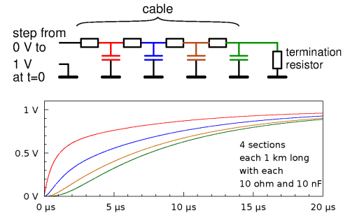
attempted to describe what happens in a long telegraph cable.
His model is sketched in the figure.
He mentally chopped the cable into short pieces, each of which has some resistance and some capacitance.
Next, he calculated what happens if at the left end one suddenly applies a voltage of say 1 volt.
The graphs show the result, for a 4 km long cable having 0.1 ohm of resistance per meter,
and 10 pF of capacitance per meter.
The cable has been divided into 4 pieces of 1 km each, so each having 100 ohm and 10 nF.
We see that the voltage on the first capacitor gradually increases to 1 volt: that’s logical,
as the capacitor gets charged via the first resistor.
The voltage on the second capacitor also gradually increases to 1 volt, but slower:
that makes sense, as it is charged from the first capacitor.
And so on.
At the right end of the cable, the voltage increases only very gradually,
and this slow increases puts a limit on how quickly Morse code signs can be sent.

However, Thomson’s model is wrong.

Heaviside’s model

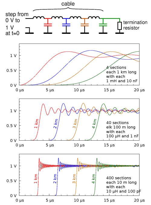
Heaviside realised that the inductance of the cable is also important.
See the next figure: here we have replaced Thomson’s resistors by inductors, of 1 µH per meter of cable length.

First have a look at the first set of graphs, marked as “4 sections”.
We see that the voltage on the first capacitor reaches the full 1 volt much earlier
than in Thomson’s model, and even overshoots.
This is because once there is current flowing in an inductor, this current doesn’t
just stop when the voltage across the coil becomes lower.
This faster increase of the voltage, and the fact that the current doesn’t just stop,
also causes the second capacitor to be charged earlier and faster than in Thomson’s model,
and so on.

Of course, modelling a 4 km long cable in just 4 pieces is not very realistic.
For a better model, we could e.g. model it using 10 times as many pieces,
each 10 times shorter (i.e., 40 pieces of 100 m each),
each with 10 times less capacitance and inductance.
The result is shown in the second set of graphs.
The third set of graphs is for a yet 10 times finer modelling of the cable.
The graphs now show the voltage at every 10th and every 100th capacitor, respectively;
i.e., still at distances of 1, 2, 3 and 4 km from the start of the cable,
like in the first set of graphs.
We see that with the more refined model, the voltages increase faster and the overshoot takes less long.

The schematic with all those coils and capacitors resembles a low-pass filter,
and indeed, we see that the voltages increase only gradually,
hinting at the absence of high frequencies.
When one partitions the model in ever smaller pieces, the inductances and capacitances
become smaller and the filter’s cut-off frequency becomes higher.
If one mathematically takes the limit, eventually modelling the cable as consisting
of infinitely many pieces, each having infinitely little inductance and capacitance,
one gets an ever more accurate model.
While doing so, the low-pass effect disappears, and the voltage jump from 0 to 1 volt
is transmitted without distortion.

Impedance

Heaviside’s model also helps us to understand what the “impedance” of a cable is.
At the left, suddenly a voltage of 1 volt is applied to the cable.
The capacitors are as yet uncharged, so there’s 1 volt across the first inductor,
causing a gradually increasing current to flow.
How large will that current become?
That depends on the inductance: the more inductance, the slower the current increases.
And it also depends on the capacitance: the more capacitance, the more charge needs to be supplied
to charge it to 1 volt.
When the capacitor has been charged to 1 volt (ignoring the overshoot),
there will be 0 volts across the inductor, so the current through it will no longer change.
The current doesn’t become 0, but remains constant, flows into the second inductor,
charges the second capacitor, and so on.

And what happens when also the last capacitor has been charged?
As noted above, the current through those inductors cannot just stop.
If we “terminate” the cable in a resistor, as shown in the figure, then the
current will flow through the resistor and cause a voltage drop across it.
If the resistor has exactly the right value, then that voltage drop is exactly 1 volt.
Then we reach a stable state: all capacitors are charged to 1 volt, across the coils
there’s no voltage, and a constant current flows from the source through the cable
and the termination resistor.

If the termination resistor is too large, the voltage drop across it will be more than 1 volt,
so the last capacitor will be charged to more than 1 volt.
Via the last inductor a part of that charge will then flow back from the last to the
second-to-last capacitor, from there to the third-last capacitor, and so on:
we get a reflected wave.
Something similar happens if the termination resistor is too small.

The value of the termination resistor which does not cause a reflection,
is called the impedance of the cable.
It turns out that this equals $\sqrt{\mathrm{<i>L/C</i>}}$,
where L and C are the inductance and capacitance per meter of cable length.
Note that this formula matches what we already observed earlier: more L means less current
and thus higher termination resistor needed to still drop 1 volt;
similarly, more C means more current and thus lower termination resistor.

Speed

In the previous figure, we effectively saw a wave move from left to right through the cable;
the farther from the source, the later the voltage change arrives.
How fast does this wave move?
That also depends on the values of L and C.
The larger the inductance L, the slower the current increases (at given voltage),
so the longer it takes to charge the next capacitor.
And the larger C, the longer it takes (at given current) to charge the capacitance.
Heaviside showed that the speed equals 1/LC.

Does this mean that we can make a cable with any desired speed,
simply by choosing L and C appropriately?
Perhaps even faster than light? (Einstein already starts turning over in his grave.)
No: it turns out that we have only limited freedom in choosing L and C.
Changing the shape and size of the cable affects both L and C, and always
such that the speed of light is never exceeded.

As an example, consider a coaxial cable.
If one makes the center conductor thinner, the capacitance between center conductor and
shield decreases, so by the formula one would expect the speed to increase.
Unfortunately, at the same time the inductance increases!
That’s (among others) because making the center conductor thinner causes the currents
inside that center conductor to be closer together, and thus sense more of each other’s
magnetic field (which, after all, is what causes (self)-inductance).

The figure shows, for a coaxial cable with air as isolation,
the theorectical dependence of the capacitance and inductance (both per meter) on the ratio of the
diameters of the center conductor and the shield.
Furthermore, the resulting impedance and wave velocity are indicated.
The solid lines are based on the assumption that the current spreads itself equally
over the entire cross-section of the center conductor.
We see that in this case the velocity increases when the center conductor is made thinner,
but does not exceed the speed of light (300 × 10⁶ m/s).
At higher frequencies the skin-effect kicks in, forcing the current to only flow on the outside
of the center conductor.
That case is indicated with dotted lines, and the speed exactly equals the speed of light,
regardless of the diameters.

If we fill the cable with e.g. some plastic material, the capacitance increases while the
inductance remains the same. Then the speed decreases; this is generally described
as the “velocity factor” being less than 1.

Loss and distortion

So far, we haven’t included loss in the model, but a real cable does have loss due to resistances,
and Heaviside included this in his model, as sketched at the right.
There are two kinds of loss.
The first one is the resistance of the copper wire itself; to model this,
Heaviside included a resistance of R ohms per meter in series with each inductance.
The second one is the leakage of the capacitor’s isolation, modelled as a parallel resistance 1/G.
(We write this as 1/G because this resistance is inversely proportional to the length;
the shorter the cable section, the less leakage, so the larger the leakage resistance.
Thus G itself, being the inverse of the resistance, is again directly proportional
to the length; it is expressed in Ω^-1 per meter, also called Siemens per meter.)

Heaviside showed that losses do not just attenuate the signal, but also cause distortion.
In fact we already saw this in Thomson’s model in the first figure:
the sudden increase of the voltage at the input of the cable, is distorted to something
that only rises slowsly, as it travels down the cable.

However, Heaviside also found out that this distortion disappears if the following
condition is satisfied: L/R = C/G.
If there is no loss, then R and G are both 0, so the condition is satisfied.
But a realistic cable usually has L/R much smaller than C/G,
because G, the leakage of the isolation, is almost zero (good isolation material),
and particularly in submarine cables, the capacitance is rather high.
In principle, we can improve such a cable in four ways to satisfy the condition:

• decrease R: use thicker copper wire, that’s expensive.
• decrease C, i.e., increase the distance between the wires: that may be feasible
  on telegraph poles on land, but making a coaxial submarine cable thicker is hard (expensive).
• increase G, so use a not-so-good isolation material: this is what happens when
  water seeps into a sea-cable (recall that Heaviside as a telegraph operator had already noticed that
  then the distortion is reduced), but the obvious disadvantage is that the signals
  become weaker.
• what remains: increase L.

Indeed, special cables have been manufactured in which the center conductor has extra
inductance, by covering it in a suitable magnetic material.
But the most commonly used way to increase L, is by connecting a coil in series
every couple of kilometers.
Heaviside invented this idea, but William Preece, the British telegraph service’s
engineer-in-chief didn’t believe it, and in fact thought that one should avoid inductance.
As a consequence, the technique initially was not tried in England (and this was not the
only conflict between Heaviside and Preece [1]).
But Michael Pupin patented the idea a few years later in America.
It turned out to work very well and has been used for decades in the telephone industry,
until it became possible to amplify signals electronically.
And radio amateurs have, particularly in the 1970s and 1980s, used such Pupin coils
for making audio filters.
The picture shows a typical Pupin coil. It had two windings, with red and green wires,
for both wires of the telephone line. Separately the windings usually were 22 mH,
in series 88 mH.

Should we now also insert coils into our antenna cables to prevent distortion of our
radio signals?
No: firstly the distortion is negligible for relatively narrow-band signals;
and secondly, such coils would work as a low-pass filter, so our (high) frequencies
wouldn’t get through anymore.

References

[1] Basil Mahon: The forgotten genius of Oliver Heaviside — A maverick of electrical science. 2017.