Time-series forecasting through recurrent topology

The main goal of time-series prediction is to collect and analyze past time-series observations to enable the development of a model that can describe the behaviour of the relevant system²⁸. SETAR models have a long history of modelling time-series observations in a variety of data types^{3,6,7,17,18,51,52,53}. They are nonlinear statistical models that have been shown to be comparable or better than many other forecasting models including some neural network-based models on real-world data^{3,6,7,17,51,52}. SETAR models also have the advantage of capturing nonlinear phenomenon that cannot be captured by linear models, thus representing a commonly used classical model for forecasting time-series data^{3,6,7,17,51,52,53}.

The most common approach for SETAR modelling is the 2-regime SETAR (2, p₁, p₂) model where p₁ and p₂ represent the autoregressive orders of the two sub-models. This model assumes that a threshold variable is chosen to be the lagged value of the time-series, and thus is linear within a regime, but is able to move between regimes as the process crosses the threshold^7,17,18. This type of model has had success with respect to numerous types of forecasting problems including macroeconomic and biological data^{3,6,7,17,51,52,53}. However, SETAR model autoregressive orders and the delay value are generally not known, and therefore need to be determined and chosen correctly⁶.

In recent years, machine-learning methods, including NNET models have attracted increasingly more attention with respect to time-series forecasting. These models have been widely used and compared to various traditional time-series models as they represent an adaptable computing framework that can be used for modelling a broad range of time-series data^6,41,43. It is therefore not surprising that NNET is becoming one of the most popular machine-learning methods for forecasting time-series data^6,43. The most widely used and often preferred model when building a NNET for modelling and forecasting time-series data is a NNET with a Multilayer Perceptron architecture given its computational efficiency and efficacy^{6,18,43,54,55} and its ability to be extended to deep learning¹. There are two critical hyperparameters that need to be chosen, the embedding dimension and the number of hidden units¹⁸. For deep learning, there is a third critical hyperparameter that also needs to be selected; the number of hidden layers. The choice of the value of hidden units depends on the data, and therefore must be selected appropriately. Perhaps the most crucial value that needs to be chosen is the embedding dimension as the determination of the autocorrelation structure of the time-series depends on this⁶. However, there is no general rule that can be followed to select the value of embedding dimension. Therefore, iterative trials are often conducted to select an optimal value of hidden units, embedding dimension, and number of hidden layers (for deep learning), after which the network is ready for training^1,6,18.

Many parameterized prediction models, including SETAR and artificial neural networks, are often limited in that performance of these models highly depends on the chosen hyperparameters such as embedding dimension, delay value, or model architecture. These types of models can also require tuning and optimization in high-dimensional parameter space which can have an impact on model selection, performance, and system-level constraints such as cost, computational time, and budget²³. Thus, the motivation for this work was to overcome these drawbacks and develop a simple, yet effective general-purpose algorithm with no free parameters, hyperparameter tuning, or critical model assumptions. The algorithm is based on identifying recurrent topological structures that can be used to forecast upcoming dynamic changes and is introduced next.

Forecasting through Recurrent Topology (FReT)

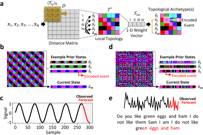
As dynamic systems can exhibit topological structures that may allow predictions of the system’s time evolution^11,56, an algorithm that can reveal unique topological patterning in the form of memory traces embedded in a signal may offer an approach for dynamical system forecasting. Local topological recurrence analysis is an analytical method for revealing emergent recurring patterns in a signal’s surface topology⁴⁰. It has been shown to be capable of outperforming neural network-based models in revealing digital biomarkers in time-series data⁴⁰, and may therefore offer a computational tool to decode topological events that may reflect a system’s upcoming dynamic changes. However, to be able to forecast based on recurring local topological patterning, we would first need to find prior states that share overlapping recurring patterns with respect to the system’s current state. Importantly, we need to be able to do this using a 1-D time-series. This would eliminate the need for time-delay embedding hyperparameters and the uncertainty associated with their estimation. If these overlapping recurring patterns, or archetypes, can be identified, they could be used for decoding complex system behaviours relevant to a dynamic system’s current state, and thus its expected future behaviour.

For instance, consider a data sequence where \({{{{{\rm{x}}}}}}\) represents a 1-D time-series vector with \({x}_{n}\) indexing the system’s current state:

With local topology, this 1-D signal is transformed into a local 3 × 3 neighbourhood topological map based on the signal’s distance matrix:

where \({D}_{{ij}}\) represent the elements of the \(n\times n\) Euclidean distance matrix. This approach represents a general-purpose algorithm that works directly on 1-D signals where the 3 × 3 neighbourhood represents a local point-pair’s closest surrounding neighbours⁴⁰. While different neighbourhood sizes can be used, a 3 × 3 neighbourhood provides maximal resolution. The signal’s local topological features are then captured by different inequality patterning around the 3 × 3 neighbourhood when computed for all \({T}_{{ij}}\) by constructing the matrix (\({T{{\hbox{‘}}}}\)) that represents an 8-bit binary code for each point-pair’s local neighbourhood:

Here g₀ represents \(({D}_{{ij}})\) and \({g}_{q}=\{{g}_{1},\ldots ,{g}_{8}\}\) are its eight-connected neighbours⁴⁰. Each neighbour that is larger or equal to g₀ is set to 1, otherwise 0. A binary code is created by moving around the central point g₀ where a single integer value is calculated based on the sum of the binary code elements (0 or 1) multiplied by the eight 2^p positional weights. This represents 8-bit binary coding where there are 2⁸ (256) different possible integer values, ranging from 0 to 255, that are sensitive to graded changes in surface curvature of a dynamic signal⁴⁰. The range is then divided into sextiles to create 6 integer bins that are flattened into a 2-D matrix (Fig. 1) where this 2-D \(m\times m\) matrix (\(m=n-2\)) can be thought of as a set of integer row vectors (\({\mathop{x}\limits^{ \rightharpoonup }}_{i}\)) with the last row vector (\({\mathop{x}\limits^{ \rightharpoonup }}_{m}\)) representing the system’s current state. We can then determine the similarity of \({\mathop{x}\limits^{ \rightharpoonup }}_{m}\) to all other prior states, \({\mathop{x}\limits^{ \rightharpoonup }}_{i}\):

using a simple Boolean logic-based similarity metric \({S}_{{im}}\):

Here, each element-wise difference in row vectors \({\mathop{x}\limits^{ \rightharpoonup }}_{m}\) and \({\mathop{x}\limits^{ \rightharpoonup }}_{i}\) are computed, generating a 1 (True) if their difference equals zero, otherwise 0 (False). This \({S}_{{im}}\) similarity metric, which differentially weights the importance of each part of the input data, can therefore range from 0 to 1, with values approaching 1 being weighted stronger. This produces a 1-D weight vector with respect to the system’s current state where higher values represent topological sequences that more closely align with the system’s current state (e.g., Supplementary Movie 1). The operations associated with Eqs. 2 and 3 are therefore important as they enable local contextual information to distinguish between signal data points with similar scalar values. In other words, they help reveal archetypes based on topological sequence patterning rather than the closest points in state space which requires the assumption that future behaviour varies smoothy.

We can now define a set of \({S}_{{im}}\) threshold values ranging from around 0.6 to 1.0 with which to maximize to find \({\mathop{s}\limits^{ \rightharpoonup }}_{i}\), a row vector from the set of all \({\mathop{x}\limits^{ \rightharpoonup }}_{i}\) that is highly similar to the local topology state changes of the system’s current state, \({\mathop{x}\limits^{ \rightharpoonup }}_{m}\):

Thus, topological archetype detection effectively reduces to a simple maximization problem where the row index of \({\mathop{s}\limits^{ \rightharpoonup }}_{i}\) + 3 (to account for the \(m\times m\) matrix dimensions and a forecast starting at \(n\) + 1 in the future) equals the index of the encoded archetype in \({{{{{\rm{x}}}}}}\) (Eq. 1). In principle, threshold maximization will find the archetype (row vector) with greatest similarity. However, for more robust point estimates, we can subject the maximization to the constraint: a minimum of ≥3 \({\mathop{s}\limits^{ \rightharpoonup }}_{i}\). This was used in this study unless otherwise stated. Under this condition, the element-wise average of the signal trajectory extending out from the encoded regions are used to model the forecast, where the standard error can be used as a metric of uncertainty. For nonstationary long-run mean data, the encoded signal is first centred before the element-wise average is computed, and the modelled forecast remapped to the current state by adding the difference between the last data point of the series and the first point of the centred forecast.

Datasets

For the initial illustrative examples, a simple sine wave was constructed by a sequence of 300 points ranging from 0.1 to 30 with an interval of 0.1. For the string of text, a well-known Dr. Seuss book excerpt that has been used for time-series analysis was used⁵⁷. For more complex dynamic systems, the Rössler (a = 0.38, b = 0.4, c = 4.82, and ∆t = 0.1) and Lorenz (r = 28, σ = 10, \(\beta\) = 8/3, and ∆t = 0.03) attractor systems were used with initial parameters based on previous values^10,25. Every second data point was used for analysis of these time-series, so the same duration was covered, but with only half the data points. The publicly available embedded versions of the Mackey-Glass time-series were also used in this study²⁷.

Both the population and macroeconomic datasets used in this study are available in R^4,18,29. The lynx data consists of the annual record of the number of Canadian lynx trapped in the Mackenzie River district of North-West Canada for the period 1821-1934^4,18. The macroeconomic datasets used here correspond to the U.S.-Canadian dollar exchange rate from 1973 to 1999^18,29, and the month U.S. unemployment rate from January 1948 to March 2004^18,30.

Gait data were analyzed from a heterogeneous sample of five young to middle-aged adults without gait impairment⁴⁰ using a single wearable sensor⁵⁸. The sensor system is based on using motion processor data consisting of a 3-axis Micro-Electro-Mechanical Systems (MEMS)-based gyroscope and a 3-axis accelerometer. The system’s firmware uses fusion codes for automatic gravity calibrations and real-time angle output (pitch, roll, and yaw). The associated software application utilizes sensor output for gait biometric calculations in real-time while recording gait-cycle dynamics and controlling for angular excursion and drift^58,59,60. The sensor is attached to the leg just above the patellofemoral joint line through the use of a high-performance thigh band which is the optimal location for this sensor system^58,59,60.

Data analysis

In addition to recent benchmark data generated in the literature, SETAR, NNET, and D-NNET models were also used for FReT comparative analysis. For the SETAR models, different forecasting methods were used for testing (Naïve, Bootstrap resampling, Block-bootstrap resampling, and Monte-Carlo resampling)¹⁸. For macroeconomic model building, a logarithmic transformation (log10) was first applied to the data as commonly done⁶¹. Specific model details and network architectures are noted when presented. For FReT, data were log-transformed after forecasting to enable comparison to SETAR, NNET, and D-NNET models.